TikzDevice tutorial III: standalone plots

In this post I’m going to show you how to use tikzDevice to create high quality plots that use the same font as your \(\LaTeX\) document. I’m assuming that you have already installed tikz. If not, see part I in this series. Moreover, this tutorial assumes that you have set up your project in the same way outlined in part II. An added benefit to this approach is that it allows you to insert IPA symbols into the plot via the tipa package.

The LaTeX file

Ok. You should start with a \(\LaTeX\) file that looks like this:

\documentclass{article}
\usepackage{tikz}
\usepackage{tipa}

\begin{document}

<<>>=
require(tikzDevice)
tikz('plot.tex', standAlone=TRUE)
library(stats)
plot(cars)
lines(lowess(cars))
dev.off()
@

\end{document}

If you have experience working with \(\LaTeX\), the preamble should be pretty straightforward (If you need a quick primer on \(\LaTeX\), see this tutorial). The important part so far is that you have to include \usepackage{tikz} and \usepackage{tipa} before \begin{document}.

The R code

In knitr, R code goes between <<>>= and ends with @. So all of this is R code:

require(tikzDevice)
tikz('plots/cars-plot.tex', standAlone=TRUE)
library(stats)
plot(cars)
lines(lowess(cars))
dev.off()

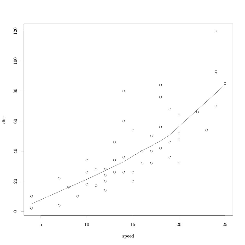
The command require(tikzDevice) loads tikz into the R workspace. Then, tikz('plots/cars-plot.tex', standAlone=TRUE) calls the tikz device and creates the file cars-plot.tex in the folder plots. It is important to set standAlone to TRUE if you want to have a separate .tex file (this is what allows us to keep the fonts the same as the rest of the document). From this point on until the call dev.off(), we enter what we want to appear in our .tex file. In this case I have plotted the typical cars data from the library stats. Here is the PDF output produced when cars-plot.tex is compiled. Notice the font is different from what you typical get in R.

Now let’s try something a little more involved and add some IPA. I will use a fake dataset and load it into R.

my_data <- read.delim("assets/my_data.txt")

We will use ggplot2 for this plot.

library(ggplot2)

Now we will call tikz device.

require(tikzDevice)
options(tikzLatexPackages = c(getOption("tikzLatexPackages"), "\\usepackage{tipa}"))
tikz('plots/ipa_plot.tex', standAlone=TRUE, width=10, height=6)
my_data$group <- factor(my_data$group, levels = c("EL", "NE", "LL"))
df<-with(my_data, aggregate(fpro, list(group=group, fstim=fstim), mean))
df$se<-with(my_data, aggregate(fpro, list(group=group, fstim=fstim), function(x) sd(x)/sqrt(10)))[,3]
gp <- ggplot(df, aes(x=fstim, y=x, colour=group, ymin=x-se, ymax=x+se))
gp + geom_line(aes(linetype=group), size = .5) + 
    geom_point(aes(shape=group)) + 
    geom_ribbon(alpha = 0.15, linetype=0) + 
    ylim(0, 1) + 
    scale_x_continuous(breaks=seq(0, 10, by=1)) +
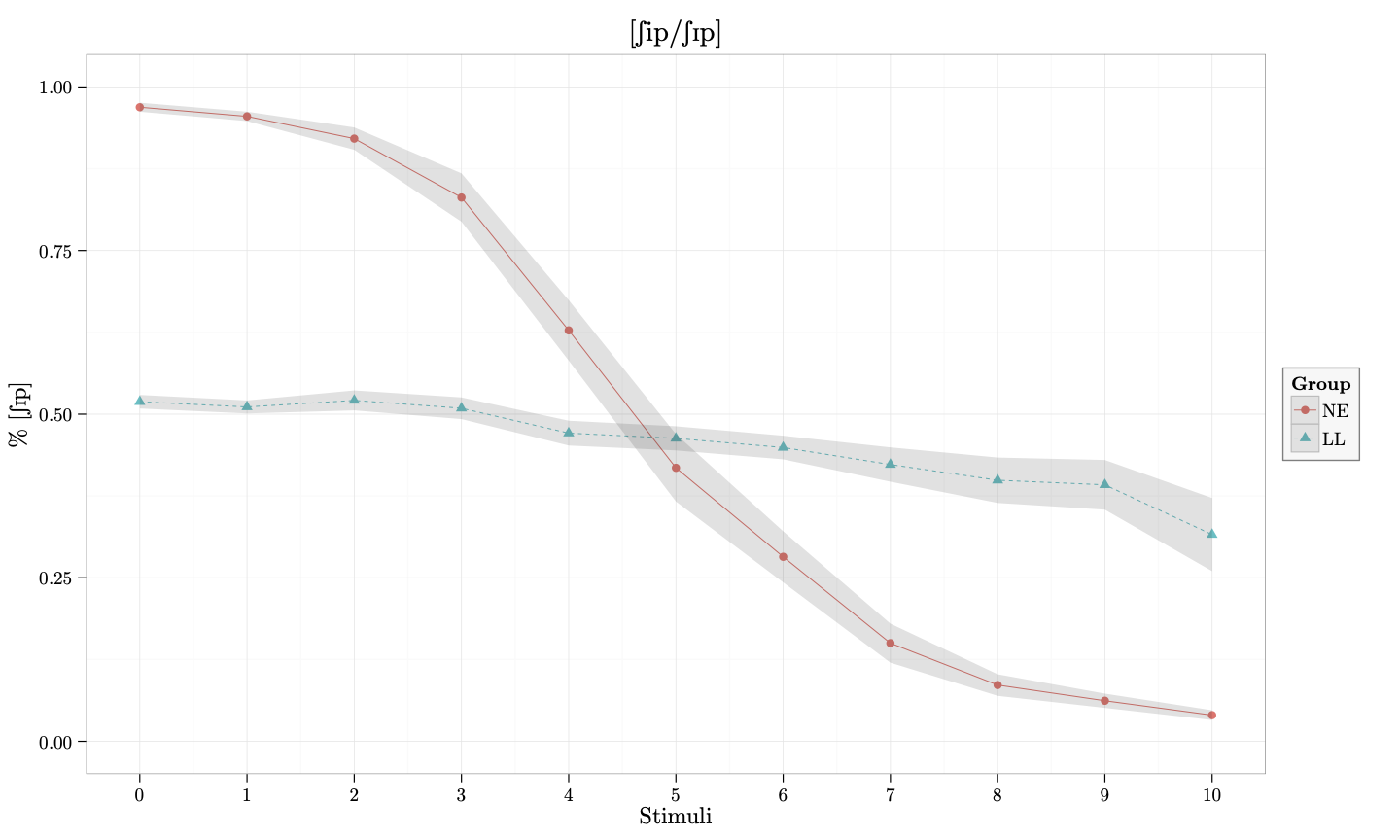
    labs(list(title = "[\\textesh ip/\\textesh\\textsci p]", 
            x = "Stimuli", y = "\\% [\\textesh\\textsci p]")) +
    theme_bw() +
    theme(legend.background = element_rect(colour = 'grey50', 
        fill = 'grey97', size = .75, linetype='solid')) +
    scale_linetype_discrete("Group") +
    scale_shape_discrete("Group") +
    scale_colour_discrete("Group")
dev.off()

Notice that after the require(tikzDevice) call, we included

options(tikzLatexPackages = c(getOption("tikzLatexPackages"), "\\usepackage{tipa}")) 

The key component here is \\usepackage{tipa}. This means that tipa will be included in the .tex produced from the code, which, in turn, means that we can include IPA sybols in the plot before it is produced. The tikz('plots/ipa_plot.tex', standAlone=TRUE, width=5, height=5) call creates ipa_plot.tex in the folder plots. The rest of the code (up to dev.off()) is the actual plot. Notice that we have included ipa in the following command:

labs(list(title = "[\\textesh ip/\\textesh\\textsci p]", 
          x = "Stimuli", y = "\\% [\\textesh\\textsci p]"))

This is the plot that is produced when the resulting .tex file is compiled:

And that’s it. We have produced a beautiful plot that uses the same font as our document and includes IPA symbols. You can download all the files here and try it yourself.